CENTAR » Example

Tools: SPADE LU Decomposition Example

1. Algorithm Derivation

Here LU decomposition is used as an example to show in detail how arrays can be derived directly from mathematical expressions. LU decomposition also serves as a useful benchmark in comparing previous tool and methodology efforts because many of these use it as an example. Here it will be shown how little user intervention is required in the design process and how easy it is for a circuit designer to easily explore a variety of array implementation tradeoffs.

Given a linear system Ax=b, where A is a known NxN matrix , b is a known vector, and x is an unknown vector, a common solution is to decompose A into a product of two matrices, one lower triangular in form (L) and the other upper triangular (U), so that LUx=b. This allows the linear system to be decomposed into two easier to solve systems,

$\small \begin{matrix} Ly=b\\ Ux=y \end{matrix}$

where another another unknown vector y has been introduced. Each equation above can then be solved by the process of “back substitution”. For example, Ly=b can be written in the matrix form

$\small \begin{bmatrix} l_{11} & 0& 0\\ l_{21} & l_{22}& 0\\ l_{31}& l_{32} & l_{33} \end{bmatrix} \begin{bmatrix} y_{1}\\ y_{2}\\ y_{3} \end{bmatrix} = \begin{bmatrix} b_{1}\\ b_{2}\\ b_{3} \end{bmatrix}$

whereupon it can be seen that three recursive expressions in y allow the solution

$\small \begin{bmatrix} y_{1}=b_{1}/l_{11}\\ y_{2}=b_{2}-l_{21}y_{1}\\ y_{3}=b_{3}-l_{31}y_{1}-l_{32}y_{2} \end{bmatrix}$

or in general for L

$\small y_{i}=b_{i}-\sum_{k=1}^{i-1}l_{ik}y_{k}$

A similar expression provides the solution x now that y is known. Thus, using this approach, all that is required to solve the linear system is to decompose A into the product LU. Such a decomposition can be done in a fashion similar to that above, which can be seen directly from the form

$\small \small \begin{bmatrix} l_{11} & 0& 0\\ l_{21} & l_{22}& 0\\ l_{31}& l_{32} & l_{33} \end{bmatrix} \begin{bmatrix} 1 & u_{12}& u_{13}\\ 0 & 0& u_{23}\\ 0 & 0 & 1 \end{bmatrix} = \begin{bmatrix} a_{11} & a_{12}& a_{13}\\ a_{21} & a_{22} & a_{23}\\ a_{31} & a_{32} & a_{33} \end{bmatrix}$

Hence, it can be determined by induction that

$\small \begin{matrix} l_{11}=a_{11};\; l_{21}=a_{21};\; l_{31}=a_{31};\\ u_{12}=a_{12}/l_{11};\; u_{13}=a_{13}/l_{11};\\ and\: for\:\: i\geq j,\: j>1\: i\leq 3;\\ l_{ij}=a_{ij}-\sum_{k=1}^{j-1}l_{i,k}u_{k,j}\\ and\: for\:\: j> i,\: i>1\: j\leq 3;\\ u_{ij}=\left ( a_{ij}-\sum_{k=1}^{j-1}l_{i,k}u_{k,j} \right )/l_{ij} \end{matrix}$

From the mathematical expression in above it is possible to go directly to the code form:

for i to N do
      for j to N do
          if j=1 and i>=1 and i<=N then
              l[i,j]:=a[i,j];
          elif i=1 and j>1 and j<=N the
              u[i,j]:=a[i,j]/l[i,i];
          fi;
          if i>=j and j>1 and i<=N then
              l[i,j]:=a[i,j]-add(l[i,k]*u[k,j],k=1..j-1)
          fi;
          if j>i and i>1 and j<=N then
              u[i,j]:=(a[i,j]-add(l[i,k]*u[k,j],k=1..i-1))/l[i,i]
          fi;
      od
od;

Here, the only semantic change has been to use the Maple “add” construct in the place of the mathematical summation sign. Also, N replaces “3″ and is a measure of the “problem size”. In this example it is possible to run this code directly in Maple to verify it’s functionality.

This code is saved as a text file and read into SPADE as a text file at the beginning of processing by the parser. All variables are required to be indexed and of dimension less than three. There is nothing in the space-time mapping methodology that imposes this limitation; rather it was a practical choice based on the observation that this covers most signal processing algorithms of choice.

The FFT design proceeds in the same way with inputs to SPADE derived from first principles. In general there are no steps in the process involving detailed issues related to parallel algorithms or relating to architectural implementation issues. Many other signal processing examples, including the FFT, are provided in the reference links.

2. LU Decomposition Design Results

A critical tool function is to provide the circuit designer with a complete range of architectural options so that tradeoffs can be adequately analyzed. This is necessary because available FPGA/ASIC chips, boards and virtual computers are built with different architectural features and any system implementation based on such technologies will have its own unique set of constraints. The examples below show how such considerations can result in very different array (abstract circuit) designs.

2.1 Input Constrained to Array Boundary

In this first mapping example the architectural constraints were set to require all input to take place from the systolic array boundary and look for the minimum time latency solution that has the least PE array area. (In this case variable a is the input.) It is a common characteristic of systolic arrays, which are physically tied to sensors to have sensor data stream into the array from one or more array edge boundaries, and also consistent with FPGA based virtual computers that contain a lot of buffer memory at the board inputs.

With the LU decomposition input code above the parser analysis generates 55 search variables that are uniquely associated with the scheduling operation. However, the causality constraints and other high level architectural constraints reduce the number of these search variables to 19. There are also 6 unimodular matrices associated with the reindexing step that in part specifies S, and these matrices must be chosen from a set, typically less than 50. When all high level constraints applied, the search space of possible mappings is reduced to a range that can be explored in a reasonable length of time.

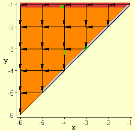
Figure 1. The first of two mappings for LU decomposition with input variable a constrained to appear on the array boundary (N=6). (Variable l is orange, u is grey and a is red.)

The search discovered 303 solutions that satisfied causality. These can be grouped into just 2 time latency categories proportional to 3N and 4N. However, when additive constants are considered (e.g., 4N-3) there were 8 distinct latency values for all solutions. Constraints associated with the boundary I/O and reindexing reduced the total number of feasible solutions to 14 and finally after all constraints were considered there were only six unique mappings with the minimum time latency of 3N-3. These array designs were all triangular in shape. Four of these had less desirable “diagonal” interconnection patterns between PEs. Going through the search process again with the secondary constraint set to find the most regular solutions, yielded just two designs that have the more desired “rectangular” interconnect structure. These two designs are shown in Figures 1 and 2 for the case where N=6.

Here, as with later mappings, the x and y axes represent the spatial coordinates of a 2-D mesh grid with the array of PEs embedded in this grid at intersection points. The grid above is NxN in size and the embedded systolic array is triangular with N(N+1)/2 PEs. The different shadings correspond to regions associated with the different algorithm variables a, l and u and are labeled as such.

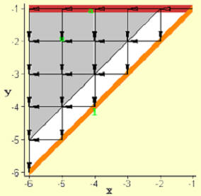
Figure 2. The second of two mappings for LU decomposition with input variable a constrained to appear on the array boundary (N=6).

The PE arrays in Figure 1 and 2 are uniform in terms of the interconnection pattern and there are six different flows of data associated with the various variable dependencies, each of which moves along an orthogonal path defined by the arrows in Figure 1 and 2. Thus, some PEs experience six different data streams passing through them. There are three additional dependencies in which data does not move spatially, but rather is updated and reused in the same PE. This corresponds to data “movement” along the time axis in space-time. The picture in Figures 1 and 2 show a superposition of data flow at all times. The actual time variation of data flow is more complex, with the size of uniform sub-regions of PEs growing and shrinking with time. In other words data movement typically begins at one edge of the array and proceeds outwards in a “wavefront-like” fashion.

In space-time all three algorithm variables, a,u and l, are represented by polygons because they are defined with two indices in the algorithm code above. That is, the index points in space-time to which the element values a[i,j], u[i,j] and l[i,j] are mapped lie on a planar surface. When the normal to these surfaces is perpendicular to the time axis, they are projected onto the 2-D mesh array as lines as shown in Figures 1 and 2. In this first mapping example such a constraint was only placed on certain search variables associated with the elements of input variable a. (The boundary alignments of u in Figure 1 and l in Figure 2 occurred only because these lead to the most regular array.)

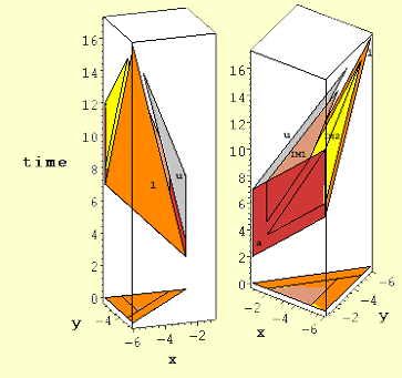
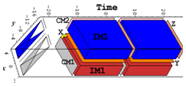
Figure 3. Position of algorithm variables u, l, and a in space-time for two different orientations.
Projection of these surfaces along the time axis yields the triangular array of Figure 1.
The outline of this projection is shown here at time=0.

SPADE also provides a space-time view of each algorithm array mapping solution, one of which is shown in Figure 3 and corresponds to the spatial-only view in Figure 1. The space-time view is shown from two different perspectives in order to help in its interpretation (in the SPADE environment this view can be easily manipulated along all axes in real-time).

Figure 3 is more complex because it shows additional variables, IM1 and IM2 (IM1[i,j,k]=l[i,k]*u[k,j]; IM2 has the same dependence on l and u, but a different index domain and both are polytopes in the space-time view and are not seen in the original algorithm code above. These two new variables are created automatically in the parser and are there to keep running sums associated with the summations.

This view imparts a good deal more information than the spatial view. For example it shows where and when array activity associated with the different algorithm variables takes place, it provides a visible view of 3-D data flow between algorithm variables, and it imparts a rough estimate of how efficiently PEs are used by what percent of the total space-time volume is occupied by polytopes and polygons.

In Figure 3, it can perhaps been seen more clearly that the normal to the polygons representing variables a and u in space-time is in the plane of the PE array and therefore their projection on this plane is a line.

The design significance of placing a variable entirely along an edge boundary goes beyond its proximity to the rest of the system, which is external to the array. It means that each PE associated with one of the edge points on the grid must have a memory size that’s O(N), where N specifies the size of the problem. This requirement is different from PEs internal to the array for which the memory requirement is small and independent of the problem size.

Given the considerations above, the circuit designer might wonder if there is an architecture that doesn’t place either l or u at the edge of the array as in Figure 1 and 2. This could be potentially motivated by the desire to have all the output data internal to the array for subsequent processing. Such a solution does not appear amongst those that fall into the minimum area category. But by having SPADE generate some of the more sub-optimal area solutions, the desired result can be found and is shown in Figure 4. Cleary the tradeoff in accepting the array shown in Figure 4 is that it is about twice the size of the previous designs. Note that the “gap” between the l and u regions is a result of the fact that the diagonal elements of u are by definition already set to one.

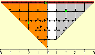
Figure 4. Array design with variables l, u not placed on array edge boundary having a time latency of 3N-3 (N=6).

2.2 Input and Output Constrained to Array Boundary

Naturally, it might be of interest as well to inquire about array designs would occur if l, u and a were all constrained to occur along the boundary. Only two solutions were found as shown in Figure 5. However, the latency of the algorithm with this new constraint has increased from the 3N-3 time steps associated with all previous designs to 4N-4 time steps. In addition the area has increased from N(N+1)/2 to (2N-1)N.

It is likely that a circuit designer would prefer working with the array design on the right in Figure 5 because here the actual PE array is square. (Sometimes it is necessary to view the SPADE space-time output in order to ascertain exactly which grid intersections of the 2-D view correspond to PEs.)

2.3 Single Divider Implementation

Although the array designs in Figure 1 and 2 look equivalent there is a significant difference between the two in terms of hardware usage. From the code above it can be seen that the line

  if j>i and i>1 ...

implies that at each point i>1,j>1, a divider is necessary to compute this statement. Consequently, in Figure 2 a triangular array of dividers corresponds to the internal shaded region labeled u, whereas in Figure 1 only a linear array associated with the linear projection of u is required for divisions.

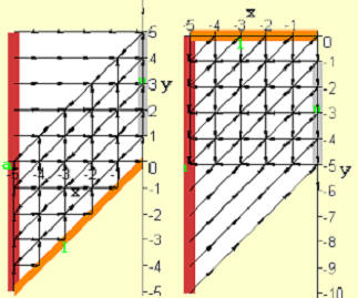
Figure 5. Two optimal arrays resulting from constraints that all input and output occur on array boundaries (N=6).

Since it is known that systolic arrays that do LU decomposition are possible that use only one divider it is useful to ask how SPADE would achieve such a result. This is best done by introduction of a new variable. This is necessary because it is clear that if a variable positioned in space-time is to project onto the spatial plane at a single point (corresponding to the divider), this variable can’t be represented by a polygon, but must be represented by a line. Hence it must be specified by a single index. Also, it is clear in the code segment

if j>i and i>1 and j<=N then
   u[i,j]:=(a[i,j]-add(l[i,k]*u[k,j],k=1..i-1))/l[i,i]
fi;

that although there are O(N²) divides associated with this statement, only N values of l[i,i] are used and this could be specified by a single index. Therefore it follows that, the number of divisions can be reduced by changing the code segment above to read

if j>i and i>1 and i<=N and j<=N then
   u[i,j]:=(a[i,j]-add(l[i,k]*u[k,j],k=1..i-1))*l_inv[i]
fi;
if i>=1 and i<=N then l_inv[i]:=1/l[i,i] fi;

and replacing instances of division by l to multiplication by l_inv elsewhere. If this change is made along with a boundary constraint on l_inv, we get the single solution shown in Figure 6 with an area of N² (minimum area secondary objective function) and time latency of 3N-3. The corresponding space-time view is shown in Figure 7 where only one PE contains a divider (upper right corner Figure 6.)

The tradeoff above is that the single divider constraint increases the array size by about a factor of two compared to the array design in Figure 1. In addition, the placement of variables l, u and a in this design might or might not be considered favorable. Also there’s data movement in nine vs the six directions for the array in Figure 1. But, while the creation of a new variable often increases the overhead in terms of data movement and computational requirements, this doesn’t happen here because the variable elements l_inv[i] remain in the same PE (no data movement) and the number of total divisions has not increased compared to previous examples.

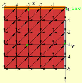
Figure 6. Optimal array implementation for single divider (upper right hand corner) (N=6).

Once an array design is selected, the actual transformation matrices are saved and available as inputs to other components of the environment; for the particular design shown in Figures 6 and 7 these are summarized in Table 1 and the dependency information (data flow vectors) is provided in Table 2.

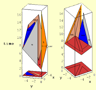
Figure 7. Space-time view of single divider array design corresponding to spatial array shown in Figure 6. Variable l_inv is the lightly shaded (yellow) vertical line at x=0, y=0.

Table 1. Transformations for array design of Figures 6 and 7.

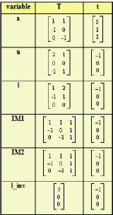
Table 2. List of direction vectors ([time,x,y]) of data flow for the Figures 6 and 7.